A basic strategy for recommendation is, find users similar to the new user, and recommend the new user with what similar users like. Based on this strategy, a technique, collaborative filtering, was invented to making predictions (filtering) about the interests of a user by collecting preferences or taste information from many similar users (collaborating).
Here we implemented a user similarity based collaborating filtering algorithm to predict ratings, and this algorithm was further applied to our shiny app.
Dependencies
library(tidyverse)
Data preparation
path = "./data/small/ratings.csv"

ratings_tidy = read_csv(path) %>%
  janitor::clean_names() %>%
  select(-timestamp)

ratings = ratings_tidy %>%
  nest(movie_id, rating)
In the data preparation process, we read the raw rating file and nested the two column movie_id and rating for following analyses’ convenience.
Algorithm
The user similarity based recommendation algorithm predict ratings with the following procedures:
- Find \(K\) most similar users to the given user (Here we set \(K\) to 10)
- Find all movies that these similar users have rated and the given user has not watched
- Predict the given user’s ratings on these movies based on the similarity measure and ratings of similar user’s
Measure of similarity
We built two functions, calc_pc_sim, calc_cos_sim, to calculate the similarity between users. In subsequent analysis, we will compare the performance of these two measure and choose the better one.
Measure by Pearson correlation
Let’s denote \(w_{uv}\) as the similarity between two users(\(u\), \(v\)), \(r\) as movie ratings, \(m\) as movie, then \(w_{uv}\) can be quantitatively defined by Pearson correlation:
\[
w_{u v}=\frac{\displaystyle \sum_{m \in M}\left(r_{u m}-\bar{r}_{u}\right) \cdot\left(r_{v m}-\bar{r}_{v}\right)}{\displaystyle \sqrt{\sum_{m \in M}\left(r_{u m}-\bar{r}_{u}\right)^{2} \sum_{m \in M}\left(r_{v m}-\bar{r}_{v}\right)^{2}}}
\]
calc_pc_sim = function(u_data, v_data){

  calc_df = u_data %>%
    inner_join(v_data, by = "movie_id", suffix = c("_u", "_v"))

  # two users should at least watched 3 same movie
  if (nrow(calc_df) < 3) {
    return(-1)
  }

  r_mean_u = u_data %>% pull(rating) %>% mean()
  r_mean_v = v_data %>% pull(rating) %>% mean()

  calc_df = calc_df %>%
    mutate(
      r_u_ct = rating_u - r_mean_u,
      r_v_ct = rating_v - r_mean_v,
      r_uv_ct = r_u_ct * r_v_ct,
      r_u_ct_sq = r_u_ct^2,
      r_v_ct_sq = r_v_ct^2
    )

  sum_r_uv_ct = calc_df %>% pull(r_uv_ct) %>% sum()
  sum_r_u_ct_sq = calc_df %>% pull(r_u_ct_sq) %>% sum()
  sum_r_v_ct_sq = calc_df %>% pull(r_v_ct_sq) %>% sum()

  sim = sum_r_uv_ct / sqrt(sum_r_u_ct_sq * sum_r_v_ct_sq)

  return(sim)
}
We built a function, calc_pc_sim, to calculate the pearson correlation according to the above formula.
Measure by cosine similarity
Alternatively, \(w_{uv}\) can also be defined by cosine similarity:
\[
w_{u v}=\frac{\displaystyle \sum_{m \in M} r_{u m} \cdot r_{v m}}{ \displaystyle \sqrt{\sum_{m \in M}r_{u m}^{2} \cdot \sum_{m \in M}r_{v m}^{2}}}
\]
calc_cos_sim = function(u_data, v_data){

  calc_df = u_data %>%
    inner_join(v_data, by = "movie_id", suffix = c("_u", "_v"))

  # two users should at least watched 3 same movie
  if (nrow(calc_df) < 3) {
    return(-1)
  }

  calc_df = calc_df %>%
    mutate(
      r_uv = rating_u * rating_v,
      r_u_sq = rating_u^2,
      r_v_sq = rating_v^2
    )

  sum_r_uv = calc_df %>% pull(r_uv) %>% sum()
  sum_r_u_sq = calc_df %>% pull(r_u_sq) %>% sum()
  sum_r_v_sq = calc_df %>% pull(r_v_sq) %>% sum()

  sim = sum_r_uv / sqrt(sum_r_u_sq * sum_r_v_sq)

  return(sim)
}
We built the function calc_cos_sim to calculate the cosine similarity according to the above formula.
Identify similar users
acquire_data = function(user){
  return(ratings %>% filter(user_id == user) %>% pull(data))
}

get_similar = function(user, calc_sim){

  user_data = acquire_data(user)
  calc_df = ratings %>%
    filter(user_id != user) %>%
    rename(v_data = data) %>%
    mutate(u_data = user_data) %>%
    mutate(
      sim = map2_dbl(u_data, v_data, calc_sim)
    ) %>%
    select(-u_data, -v_data) %>%
    arrange(desc(sim)) %>%
    head(10)

  return(calc_df)
}
We calculate the similarity score between the given user and every other users, and choose 10 users with highest similarity as similar users.
Rating prediction
Once we found users similar to the new user, we can predict the new user’s rating towards a movie \(m\) by:
\[
\hat{r}_{u m}=\bar{r}_{u}+\frac{\sum_{v \in S(u, K) \cap N(m)} w_{u v}\left(r_{v m}-\bar{r}_{v}\right)}{\sum_{v \in S(u, K) \cap N(m)}\left|w_{u v}\right|}
\]
- \(S(u, K)\): the most similar \(K\) users of \(u\)
- \(N(m)\): users who have rated on movie \(m\)
predict_rating = function(user, movie, sim_users){

  r_means = ratings_tidy %>%
    group_by(user_id) %>%
    summarize(r_mean = mean(rating))

  calc_df =
    ratings_tidy %>%
    filter(movie_id == movie) %>%
    inner_join(sim_users, by = "user_id") %>%
    left_join(r_means, by = "user_id") %>%
    mutate(
      sim_r_diff = sim * (rating - r_mean),
      abs_sim = abs(sim)
    )

  sum_sim_r_diff = calc_df %>% pull(sim_r_diff) %>% sum()
  sum_abs_sim = calc_df %>% pull(abs_sim) %>% sum()

  r_u_mean = acquire_data(user)[[1]] %>% pull(rating) %>% mean()

  rating = r_u_mean + sum_sim_r_diff/sum_abs_sim

  return(rating)
}
Test & Comparison
experiment data
set.seed(777)
experiment_data = ratings_tidy %>%
  sample_frac(0.01, weight = user_id)
Due to limited computing power, we sample 1% of all ratings data as our experiment data.
Experiment design
experiment = function(experiment_data){

  test = experiment_data %>%
    sample_frac(0.2, weight = user_id)

  train = experiment_data %>%
    anti_join(test)

  ratings_tidy = train

  ratings = ratings_tidy %>%
    nest(movie_id, rating)

  cos_sim_users =
    test %>%
    select(user_id) %>%
    distinct() %>%
    mutate(
      sim_users = map(user_id, ~get_similar(user = .x, calc_sim = calc_cos_sim))
      )

  pc_sim_users =
    test %>%
    select(user_id) %>%
    distinct() %>%
    mutate(
      sim_users = map(user_id, ~get_similar(user = .x, calc_sim = calc_pc_sim))
      )

  cos_sum_r_diff_sq_df =
    test %>%
    left_join(cos_sim_users, by = "user_id") %>%
    mutate(
      r_pred = pmap_dbl(list(user_id, movie_id, sim_users), predict_rating)
    ) %>%
    drop_na(r_pred) %>%
    mutate(
      r_diff_sq = (rating - r_pred)^2
    )

  cos_sum_r_diff_sq =
    cos_sum_r_diff_sq_df %>%
    pull(r_diff_sq) %>%
    sum(na.rm = TRUE)

  pc_sum_r_diff_sq_df =
    test %>%
    left_join(pc_sim_users, by = "user_id") %>%
    mutate(
      r_pred = pmap_dbl(list(user_id, movie_id, sim_users), predict_rating)
    ) %>%
    drop_na(r_pred) %>%
    mutate(
      r_diff_sq = (rating - r_pred)^2
    )

  pc_sum_r_diff_sq =
    pc_sum_r_diff_sq_df %>%
    pull(r_diff_sq) %>%
    sum(na.rm = TRUE)

  cos_rmse = sqrt(cos_sum_r_diff_sq) / nrow(cos_sum_r_diff_sq_df)
  pc_rmse = sqrt(pc_sum_r_diff_sq) / nrow(pc_sum_r_diff_sq_df)

  return(list(cos_rmse, pc_rmse))
}
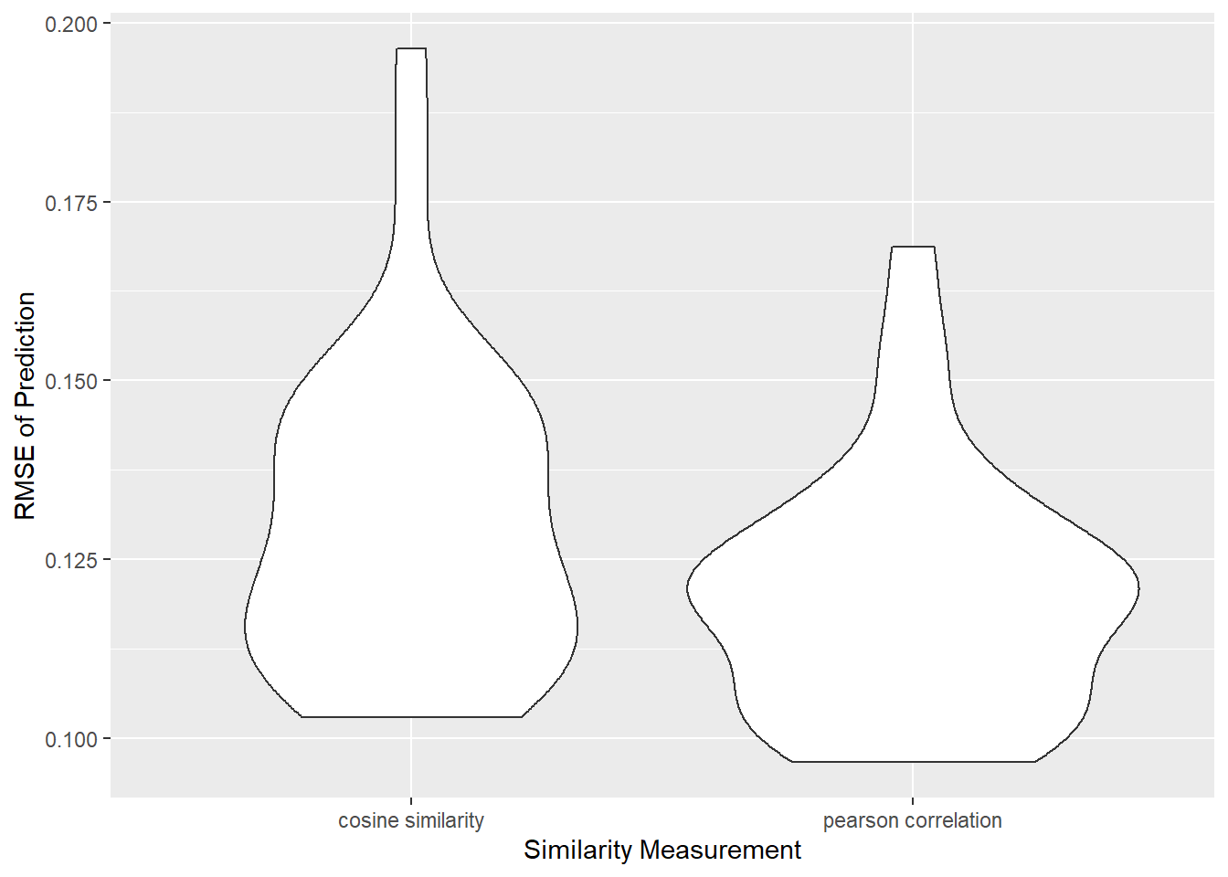
In each round of experiment, for each user, we randomly extract 20% records of their ratings as the test dataset, and the remained dataset as train dataset. Then, we use the two similarity measures separately to find similar users and subsequently predict ratings on corresponding movies in the test dataset. Finally, we compute the RMSE between predicted ratings and actual ratings in the test data set, and get the two RMSE values.
Compare RMSE
The experiment result reveals that choosing pearson correlation as the measure of similarity could yield lower RMSE values. Therefore, in our shiny app, we choose to use calc_pc_sim.
rmse_df = read_csv("./data/experiment_rmse.csv")

rmse_df %>%
  ggplot(aes(x = sim_type, y = rmse)) +
  geom_violin() +
  labs(x = "Similarity Measurement", y = "RMSE of Prediction")
Main function
main = function(user){

  sim_users = get_similar(user, calc_pc_sim)

  movies = sim_users %>%
    select(user_id) %>%
    left_join(ratings_tidy, by = "user_id") %>%
    distinct(movie_id) %>%
    pull(movie_id)

  calc_df = tibble(
    user_id = user,
    movie_id = movies
  )

  watched = acquire_data(user)[[1]] %>% pull(movie_id) %>% as.vector()

  rec_movies =
    calc_df %>%
    filter(!movie_id %in% watched) %>%
    mutate(
      r_pred = map2_dbl(user_id, movie_id, ~predict_rating(user = .x, movie = .y, sim_users = sim_users))
    ) %>%
    arrange(desc(r_pred)) %>%
    head(10) %>%
    select(movie_id, pred_rating = r_pred)

  return(rec_movies)
}
We built the main function to implement the whole process of recommendation. For the given user, we will find top 10 users similar to him/her, and predicts his/her ratings on movies similar users have seen yet he/she has not watched. Finally, we select 10 movies with the highest predicted rating to recommend to the user.
Test
Now, we can use the main function to recommend movies for a random user:
set.seed(777)

user = round(runif(1, 1, 610))

movies = read_csv("./data/small/movies.csv") %>%
  janitor::clean_names() %>%
  select(-genres)

main(user) %>%
  left_join(movies, by = "movie_id") %>%
  select(title, pred_rating) %>%
  kableExtra::kbl(digits = 1) %>%
  kableExtra::kable_styling(font_size = 12)
|
title
|
pred_rating
|
|
Godfather: Part II, The (1974)
|
5.6
|
|
American Pie (1999)
|
5.6
|
|
Being John Malkovich (1999)
|
5.6
|
|
Crouching Tiger, Hidden Dragon (Wo hu cang long) (2000)
|
5.2
|
|
Snatch (2000)
|
5.2
|
|
Batman (1989)
|
5.1
|
|
Seven (a.k.a. Se7en) (1995)
|
5.1
|
|
Raiders of the Lost Ark (Indiana Jones and the Raiders of the Lost Ark) (1981)
|
4.7
|
|
Minority Report (2002)
|
4.7
|
|
Gone Girl (2014)
|
4.7
|