Final Report
Haolin Zhong (hz2771), Shaocong Zhang (sz3030), Yuxuan Wang (yw3608), Boqian Li (bl2898)
Motivation
The prosperity of Internet industry enabled massive knowledge and entertainments to be accessible at one’s fingertips, making people no longer in thirst for feeds. However, massive information also trapped people into another dilemma: we got numerous choices for our limited attentions. Therefore, many Internet companies, such as Youtube, Tiktok and Bilibili, has equipped their website with personalized recommendation service in their backend to attract users’ attentions as much as possible. Curious about what’s behind the curtain, we decide to learn and implement recommendation algorithms to build our own recommendation system.
Initial questions
- What movies are both popular and highly-rated?
- Is there any significant differences in ratings of movies in different genres? (Which types of movie do people like?)
- Is there any relationship between movie ratings and movie release year? (Have movie ratings worsened in recent years?)
- For new users entering into the recommendation system, how to gain the first batch of rating information?
- For existing users, how to recommend movies to them?
Data
Source
The Dataset source used for EDA analysis is:MoiveLensdataset
MovieLens, a movie recommendation service, provided this dataset (ml-latest-small), which describes rating measured in the 5-star format and free-text tagging activities. It has 100836 ratings and 3683 tags generated by 610 users over 9742 movies between March 29, 1996 and September 24, 2018. This dataset was last updated on September 26, 2018.
Users in the dataset were chosen at random. All users chosen had rated at least 20 films. An id is assigned to each user, and no additional information is supplied.
The dataset was distributed in three files, movies.csv, ratings.csv, and tags.csv.
- “movies.csv” includes
movieId(movie ID),title(movie title) andgenres(movie genres). - “ratings.csv” contains
userId(user ID),movieId(movie ID),ratingandtimestamp(which represents the timepoint at which the rating was given). - “tag.csv” includes
userId,movieId,tag(text generated by a user to a movie) andtimestamp.
- “movies.csv” includes
Data cleaning
Data cleaning for EDA
library(tidyverse)
data_path = "./data/small/ratings.csv"

rating_tidy =
  read_csv(data_path, col_types = "ccnc") %>%
    janitor::clean_names() %>%
    select(-timestamp) %>%
    mutate(rating = as.double(rating))

high_rating =
  rating_tidy %>%
  filter(rating == 5.0)

movie_names =
  read_csv("./data/small/movies.csv") %>%
  rename(movie_id = movieId)
Data cleaning was performed for EDA. For dataset “rating.csv”, we applied the janitor::clean_names() function to make sure that everything is in lower case, and we also excluded the timestamp variable that did not related to our analysis assumption. After this step, we set up a new data frame called “rating_tidy”. Next up, we also created a new dataframe called “high_rating”, which only contains the highest rating score “5” of the “rating_tidy” dataframe. Last but not least, we renamed the variable “movieId” to movie_id for the “movie.csv” dataset and transfered it to a new data frame called “movie_names”. Other trivial data cleaning process were mentioned in the following EDA section.
Data cleaning for finding most differentiable movies
In finding most differentiable movies, we have done following data cleaning:
- extract
yearof release from the title of the movie - filter on
yearto only include movies released after 2000 - find number of ratings of each movie, and select 100 movies with most ratings
- convert numerical ratings into categorical variable which has three levels,
lover,hater,unknown
Filter movies released after 2000
cut_year = function(string){
  # str_split() returns a list with 1 element,
  # which is a vector containing splitted strings
  year_str = str_split(string, pattern = "\\(")[[1]]

  # sometimes the movie name also contains brackets,
  # so we only take the last element in the vector,
  # which must be the release year.
  year_str = str_remove(year_str[length(year_str)], "\\)")
  return(year_str)
}

movies = read_csv("./data/small/movies.csv") %>%
  janitor::clean_names() %>%
  mutate(
    year = map(title, cut_year),
    year = as.integer(year)
  ) %>%
  arrange(desc(year)) %>%
  drop_na(year) %>%
  filter(year >= 2000) %>%
  select(movie_id, year)
We built a function cut_year to extract year from title, and filtered movies released after 2000. The format of title is [movie name] ([release year]), thus we extracted year through identifying brackets in title.
Find 100 movies with most ratings
rating_tidy = read_csv("./data/small/ratings.csv", col_types = "iinc") %>%
  janitor::clean_names()


hot_movies =
  rating_tidy %>%
  count(movie_id) %>%
  # right join previous tibble to filter movies released after 2000
  right_join(movies, by = "movie_id") %>%
  arrange(desc(n)) %>%
  head(100) %>%
  arrange(movie_id) %>%
  pull(movie_id) %>%
  as_vector()
We built a data frame containing all users’ ratings on all movies, and found 100 movies with most ratings released after 2000. These movies were candidate for differentiable movies.
Convert rating into categorical variable type
The algorithm we implemented demands a variable suggest user’s attitude toward movies, which should have three levels: lover, hater, unknown. Therefore, We converted numerical ratings into this variable, type.
Generate the Cartesian product of users’ ratings on movies
rating_dscts =
  rating_tidy %>%
  select(-timestamp) %>%
  filter(movie_id %in% hot_movies) %>%
  # pivot_wider will generate a matrix of user's rating towards movies,
  # through which NA will be introduced when the user haven't seen the movie
  pivot_wider(names_from = movie_id, values_from = rating) %>%
  # by using pivot_longer to transform this matrix back to tidy data,
  # we introduced NA in the rating column, which suggest the user haven't seen the movie
  pivot_longer(cols = as.character(hot_movies), names_to = "movie_id", values_to = "rating")
For each user, the raw rating file only includes records for movies they rated. To generate a variable which can suggest that the user haven’t seen this movie, we generated the Cartesian product of users’ ratings on movies at first.
Conversion
classify = function(rating) {
  res = ""
  # if rating is NA, then the user has not seen this movie yet.
  if (is.na(rating)) {
    res = "unknown"

  # if rating > 3.5, we consider the user is a "lover" of this movie
  } else if (rating >= 3.5) {
    #
    res = "lover"

  # otherwise, we consider the user the movie's hater
  } else {
    res = "hater"
  }

  return(res)
}

user_cate =
  rating_dscts %>%
  mutate(type = map(rating, classify)) %>%
  unnest(type) %>%
  mutate(movie_id = as.numeric(movie_id))
In our exploratory analysis, we found that the median of all ratings is 3.5. Thus, if a user’s rating towards a movie is greater or equal to 3.5, we consider the user to be a “lover” of this movie, otherwise we consider the user the movie’s hater. If the rating is NA, then we know the user has not seen this movie and denote “unknown”.
Data cleaning for latent-factor-based recommendation
data_path = "./data/small/ratings.csv"

rating_tidy = read_csv(data_path, col_types = "ccnc") %>%
    janitor::clean_names() %>%
    select(-timestamp) %>%
    mutate(rating = as.double(rating))

rating_matrix = rating_tidy %>%
    pivot_wider(names_from = movie_id, values_from = rating, values_fill = 0.0) %>%
    column_to_rownames("user_id") %>%
    as.matrix()

users = rownames(rating_matrix)[1:20]
movies = colnames(rating_matrix)[1:20]

rating_matrix = rating_matrix[users, movies]
For latent-factor-based recommendation, we built a dataframe from the raw rating file. Then, we transformed the tidy data into a rating matrix, with column represent movies, rows represent users, and values in each grid represent ratings.
Due to the limitation of computing power, we only predict ratings for the first 20 users and the first 20 movies in the dataset.
Exploratory analysis
Summaries
Overview of dataset “ratings.csv”
We first imported the dataset “ratings.csv”, and applied janitor::clean_names() to made everything into lower cases. Next, we applied the summary() function to get the summary table. According to the result, for variable rating, the minimum is 0.5, the first quantile is 3, median is 3.5, mean is 3.502, the third quantile is 4 and the maximum is 5. Since userid, movieid, timestamp only represented the ID of users, id of movies and rating generated time, we chose not to analyze those three variables.
knitr::opts_chunk$set(echo = TRUE)
library(tidyverse)
library(readr)
library(ggplot2)
library(kableExtra)
library(pastecs)
library(ggpubr)
library(tm)
data_path = "./data/small/ratings.csv"
summary_df =
  read_csv(data_path, col_types = "ccnc") %>%
  janitor::clean_names() %>%
  summary(summary_df$rating) %>%
  knitr::kable() %>%
  kable_styling(bootstrap_options = c("striped")) %>%
  kableExtra::kable_styling(font_size = 12)
summary_df| user_id | movie_id | rating | timestamp | |
|---|---|---|---|---|
| Length:100836 | Length:100836 | Min. :0.500 | Length:100836 | |
| Class :character | Class :character | 1st Qu.:3.000 | Class :character | |
| Mode :character | Mode :character | Median :3.500 | Mode :character | |
| NA | NA | Mean :3.502 | NA | |
| NA | NA | 3rd Qu.:4.000 | NA | |
| NA | NA | Max. :5.000 | NA |
Overview of dataset “movies.csv”
We imported the dataset “movies.csv”, and applied janitor::clean_names() to made everything into lower cases. We also applied separate() function to separate the year of the variable “title”. Next, we count the genres by count() function. We also applied the filter() function to keep the n number lager than 1500.
data_path = "./data/small/movies.csv"

movie_descriptive =
  read_csv("./data/small/movies.csv") %>%
  janitor::clean_names() %>%
  separate(
  title, c("name", "year"), sep="\\s+(?=\\S*$)") %>%
  separate_rows(genres, sep = "[|]")

genres_count =
  movie_descriptive %>%
  group_by(genres) %>%
  count(genres) %>%
  filter(n >= 1500) %>%
  arrange(desc(n)) %>%
  knitr::kable() %>%
  kable_styling(bootstrap_options = c("striped")) %>%
  kableExtra::kable_styling(font_size = 12)

genres_count| genres | n |
|---|---|
| Drama | 4361 |
| Comedy | 3756 |
| Thriller | 1894 |
| Action | 1828 |
| Romance | 1596 |
Next, we also counted the 5 most appeared release year of movies, i.e. the 5 most prolific year for movie industry.
year_count =
  movie_descriptive %>%
  group_by(year) %>%
  count(year) %>%
  filter(n >= 690) %>%
  arrange(desc(n)) %>%
  knitr::kable() %>%
  kable_styling(bootstrap_options = c("striped")) %>%
  kableExtra::kable_styling(font_size = 12)
year_count| year | n |
|---|---|
|
|
733 |
|
|
719 |
|
|
709 |
|
|
705 |
|
|
691 |
Exploratory Statistical Analyses
Find movies receive most 5-star ratings
We first merged the “high_rating” and “movie_names” dataframes, and counted the movie_id variable and filtered movies with over 100 ratings. Next, we re-arranged rows according to the count and separated release year of movies from title as year. One interesting factis that among the 5 movies, 3 movies were released in 1994; 4 movies were released in the 90s.
data_path = "./data/small/ratings.csv"

rating_tidy =
  read_csv(data_path, col_types = "ccnc") %>%
    janitor::clean_names() %>%
    select(-timestamp) %>%
    mutate(rating = as.double(rating))

high_rating =
  rating_tidy %>%
  filter(rating == 5.0)

movie_names =
  read_csv("./data/small/movies.csv") %>%
  rename(movie_id = movieId)

high_rating_movienames =
  merge(high_rating, movie_names) %>%
  group_by(title, genres,rating) %>%
  count(movie_id) %>%
  filter(n >= 100) %>%
  select(n,title,genres,rating) %>%
  ungroup(title, genres,rating) %>%
  arrange(desc(n)) %>%
  separate(
  title, c("name", "year"), sep="\\s+(?=\\S*$)") %>%
  knitr::kable() %>%
  kable_styling(bootstrap_options = c("striped")) %>%
  kableExtra::kable_styling(font_size = 12)

high_rating_movienames | n | name | year | genres | rating |
|---|---|---|---|---|
| 153 | Shawshank Redemption, The |
|
Crime|Drama | 5 |
| 123 | Pulp Fiction |
|
Comedy|Crime|Drama|Thriller | 5 |
| 116 | Forrest Gump |
|
Comedy|Drama|Romance|War | 5 |
| 109 | Matrix, The |
|
Action|Sci-Fi|Thriller | 5 |
| 104 | Star Wars: Episode IV - A New Hope |
|
Action|Adventure|Sci-Fi | 5 |
Find the average rating of each genres in different year
As to find out the average rating of each genres in different year, we used separate() to separate the combined genre. Then, we found the average rating in different genres by using group_by() and summarize(). Here we only display the first ten rows of this dataframe:
movie_names_ave =
  read_csv("./data/small/movies.csv") %>%
  rename(movie_id = movieId) %>%
  separate(
  title, c("name", "year"), sep="\\s+(?=\\S*$)") %>%
  separate_rows(genres, sep = "[|]") %>%
  filter(!genres  %in% "(no genres listed)")

filter_ratingscore =
  rating_tidy

ave_rating =
  merge(filter_ratingscore, movie_names_ave) %>%
  group_by(year,genres) %>%
  summarize(mu_rating = mean(rating)) %>%
  head(10) %>%
  knitr::kable() %>%
  kable_styling(bootstrap_options = c("striped")) %>%
  kableExtra::kable_styling(font_size = 12)
ave_rating| year | genres | mu_rating |
|---|---|---|
|
|
Action | 3.5 |
|
|
Adventure | 3.5 |
|
|
Fantasy | 3.5 |
|
|
Sci-Fi | 3.5 |
|
|
Crime | 2.5 |
|
|
Western | 2.5 |
|
|
Animation | 4.0 |
|
|
Comedy | 4.0 |
|
|
Sci-Fi | 4.0 |
|
|
Drama | 2.0 |
Kruskal-Wallis Test regarding user ID and rating
We performed Kruskal-Wallis Test to determine whether there were any statistically significant differences among each users’ mean rating. The Kruskal-Wallis H test (also known as the “one-way ANOVA on ranks”) is a rank-based nonparametric test that may be used to see if two or more groups of an independent variable on a continuous or ordinal dependent variable have statistically significant differences. This method is the nonparametric counterpart of the one-way ANOVA (Kruskal-Wallis H Test in SPSS Statistics | Procedure, output and interpretation of the output using a relevant example., 2021). We choose this method instead of ANOVA due to non-normality of ratings.
Our assumption for KW test were:
\[ \begin{align} & H_0:\mu_{0}=\mu_1=\mu_2=\mu_3=...=\mu _x \\ & H_1: \text{At least two of the mean ratings of the users are different} \end{align} \]
The result showed that the p value was less than 0.05. We can thus concluded that at 0.05 significance level, we rejected the null hypothesis and concluded that at least two of the mean ratings of the user from the 600 users were different.
ggplot(filter_ratingscore, aes(x = rating, y = ..density..)) +
geom_histogram(alpha = 0.3, bins = 30) 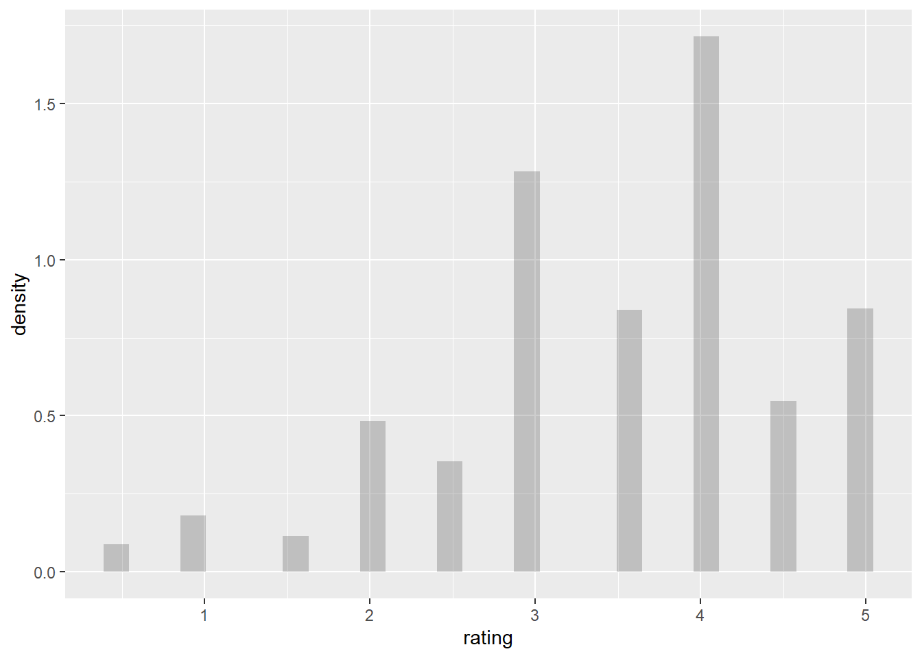
kruskal.test(rating ~ user_id, data = filter_ratingscore) %>%
 broom::tidy() %>%
 kableExtra::kbl() %>%
 kable_styling(bootstrap_options = c("striped")) %>%
kableExtra::kable_styling(font_size = 12)| statistic | p.value | parameter | method |
|---|---|---|---|
| 20676.72 | 0 | 609 | Kruskal-Wallis rank sum test |
Note: The actual p-value is less than 2.2e-16, which is too small to be shown in r. Thus, the p-value showed in the table is 0.
Visualizations
Rating distributions among different genres
After completing data cleaning process mentioned in previous sections, we merged the two dataframes, filter_ratingscore and movie_names, cleaned all column names into lower cases, extracted genres. Finally, we created a violin plot regarding ratings and genres. The plot showed that there is no obvious difference in ratings distributions among different genres.
movie_names =
  read_csv("./data/small/movies.csv") %>%
  rename(movie_id = movieId) %>%
  separate(
  title, c("name", "year"), sep="\\s+(?=\\S*$)")

filter_ratingscore =
  rating_tidy

violin_df =
  merge(filter_ratingscore, movie_names) %>%
  janitor::clean_names() %>%
  separate_rows(genres, sep = "[|]") %>%
  filter(!genres  %in% "(no genres listed)") %>%
  ggplot(aes(x = rating, y = genres)) + geom_violin(aes(color = genres, alpha = .5)) +
  theme(legend.position="none")
  viridis::scale_color_viridis(discrete = TRUE)

violin_df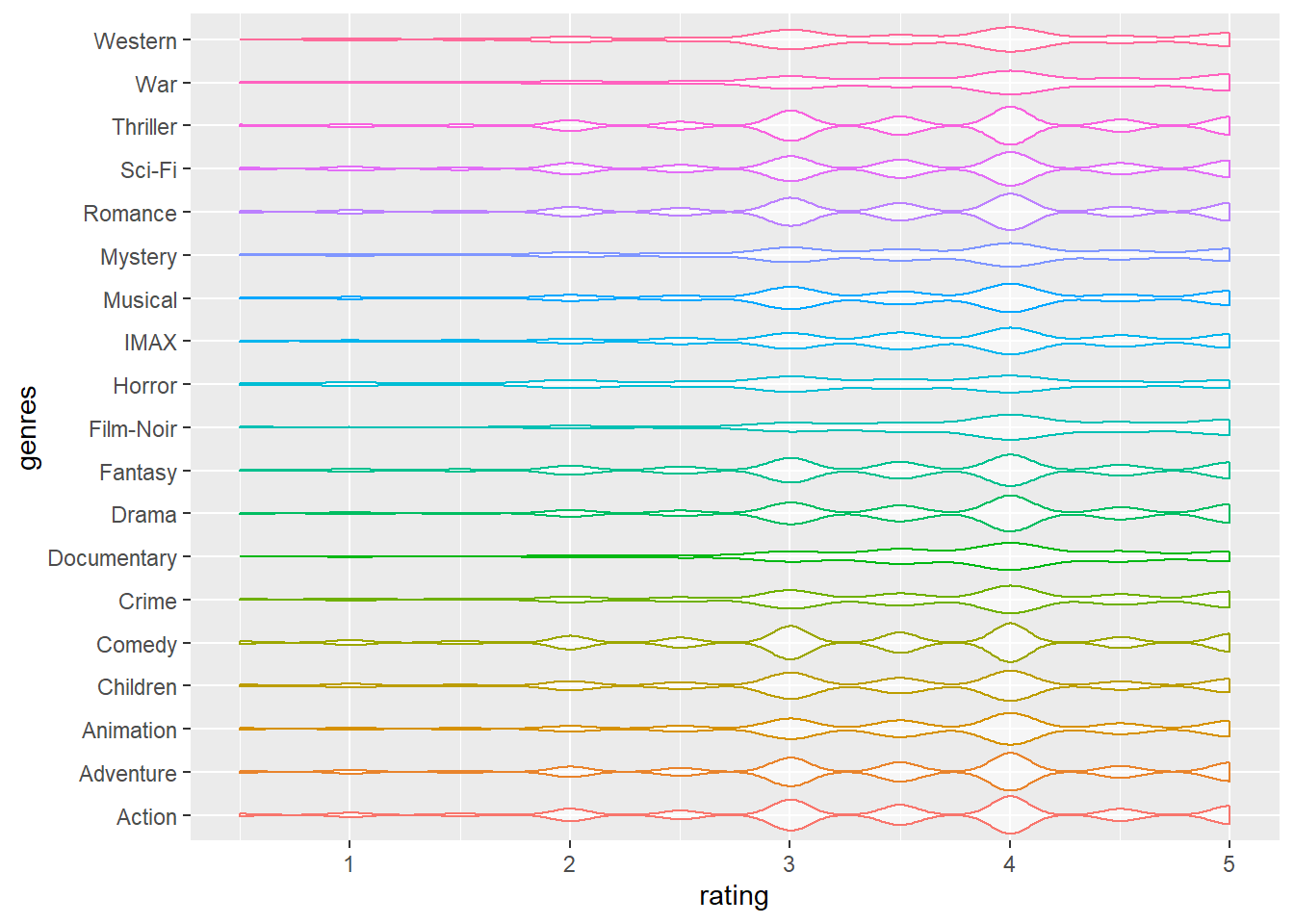
Rating distribution among different years
<<<<<<< HEAD After completing data cleaning process mentioned in previous sections, we removed brackets in year, and only included movies released between 1990 and 2018. We made a violin plot to show the rating distributions among movie release years. We found an obvious trend that from 1990 to 2018, the average rating score of movies has become more and more “similar”. That is, the rating values of modern movies are more frequently concentrated between 3.5 and 4, and the density of corresponding scores is close. However, compared to the modern movies from 2000, the user preference for movies from the 90s is more divided, and the density between different ratings is more obvious. ======= After completing data cleaning process mentioned in previous sections, we removed brackets in year, and only included movies released between 1990 and 2018. We made a violin plot to show the rating distributions among movie release years. >>>>>>> ccdb696ddc417fdb6faaa695f7a0e8a689e7e0e6
movie_names =
  read_csv("./data/small/movies.csv") %>%
  rename(movie_id = movieId) %>%
  separate(
  title, c("name", "year"), sep="\\s+(?=\\S*$)")

selected_years = 1990:2018

violin_df2 =
  merge(filter_ratingscore, movie_names) %>%
  mutate(
    year = removePunctuation(year)
  ) %>%
  filter(year %in% selected_years) %>%
  ggplot(aes(x = rating, y = year)) +
  geom_violin(aes(color = year))+
  theme(legend.position="none")
  viridis::scale_fill_viridis(discrete = TRUE)

violin_df2 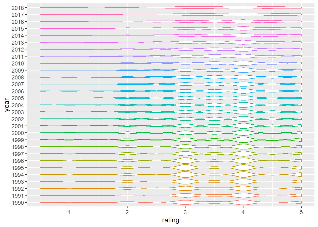
Additional analyses
Identification of differentiable movies
We implemented adaptive bootstrapping algorithm (Golbandi, N., et al. 2011) to find movies significantly differentiate people of different taste.
According to user’s response to the given movie, the algorithm classifies users into three sub-groups: lovers \(N^{+}\), haters \(N^{-}\), and people unknown of the movie \(\overline{N}\). We choose 3.5 as the cut-off to determine whether users are lovers or haters, as our exploratory analysis found that 3.5 is the median of all ratings.
The algorithm defined a term \(D_{m}\), which is equal to the sum of subgroups’ standard deviation of ratings on other movies (\(\space D(m) = \sigma_{u \in N^{+}(m)} + \sigma_{u \in N^{-}(m)} + \sigma_{u \in \overline{N}(m)} \space\)), to measure movies’ differentiation ability. By the definition, the most differential movie, i.e. the best splitter, should have the lowest \(D_{m}\), because bad splitters will divide people with different taste into the same sub-group, resulting in increased \(D_{m}\).
Once the algorithm found the most differential movie for overall users, it will repeat the above process in the 3 sub-groups, Lovers, haters and people unknown of this movie, separately. This recursive process was thus named bootstrapping. Subsequently, the algorithm will build a structure similar to a decision tree whose nodes are movies. Our implementation constructed such a ternary tree structure with a depth of 3. The result can be interpreted by the figure below:
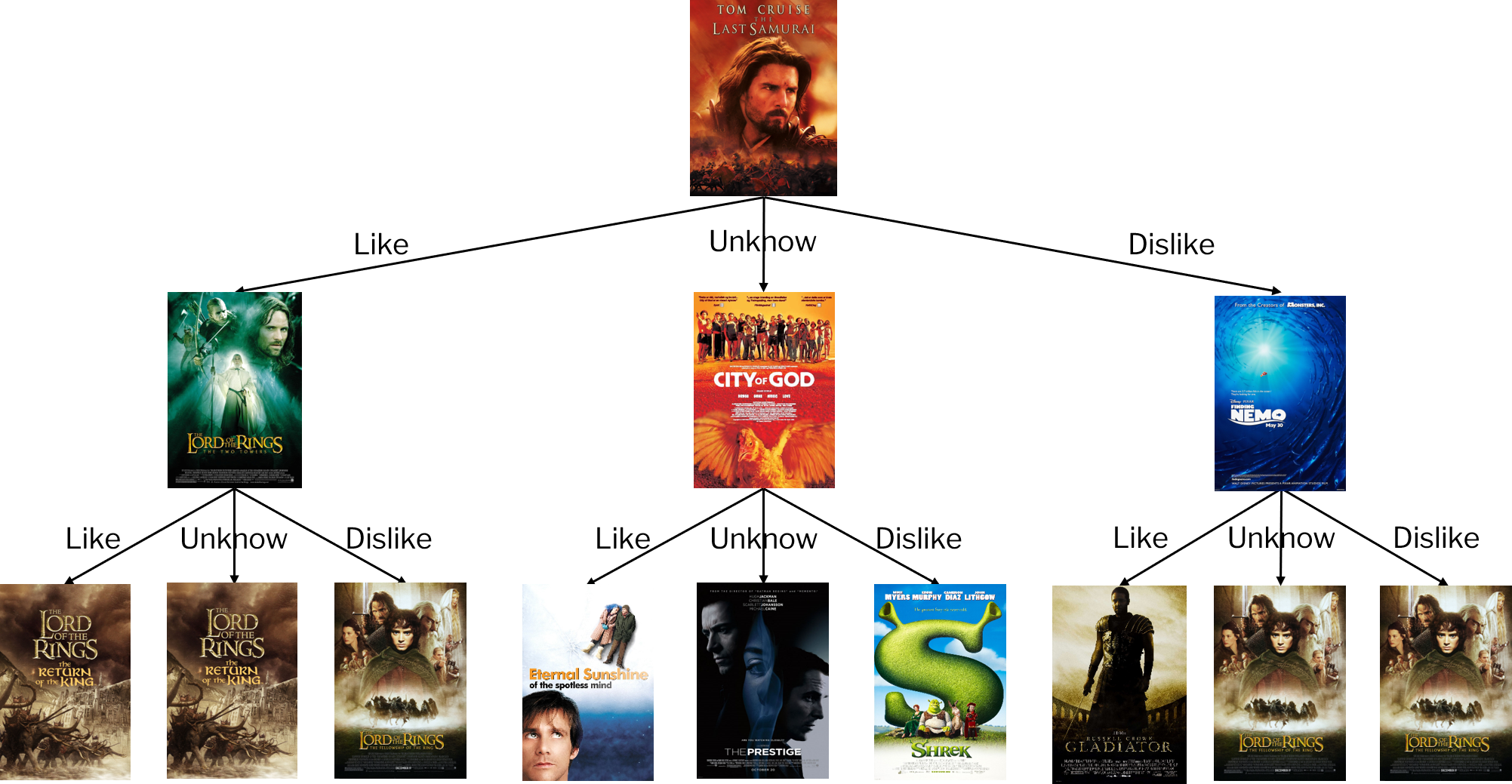
For new users, let them rate on “The Last Samurai” at first. Users who give ratings above or equal to 3.5 are considered to be lovers, and those who give ratings below 3.5 are considered to be haters. Users can also reply that they haven’t watched this movie. For lovers, we then let them rate on “The Lord of the Rings: The Two Towers”, for haters we let them rate on “Finding Nemo”, and the unknown will be asked to rate on “City of God”. After rating on the second provided movie, users will then be asked to rate on the third movie which is also adaptively provided.
Since these movies significantly differentiate people of different taste, collection of user’s rating on them will allow us to generate more personalized recommendation.
User-similarity-based recommendation
A basic strategy for recommendation is, find users similar to the new user, and recommend the new user with what similar users like. Based on this strategy, a technique, collaborative filtering, was invented to making predictions (filtering) about the interests of a user by collecting preferences or taste information from many similar users (collaborating).
This algorithm predict ratings with the following procedures: - Find K most similar users to the given user (Here we set K to 10) - Find all movies that these similar users have rated and the given user has not watched - Predict the given user’s ratings on these movies based on the similarity measure and ratings of similar users. The formula is:
\[ \hat{r}_{u m}=\bar{r}_{u}+\frac{\sum_{v \in S(u, K) \cap N(m)} w_{u v}\left(r_{v m}-\bar{r}_{v}\right)}{\sum_{v \in S(u, K) \cap N(m)}\left|w_{u v}\right|} \]
In the above process, finding similar users and predicting ratings involve the measurement of similarity, \(w_{uv}\). We considered two measurements, cosine similarity and Pearson correlation, and compared their performance through experimentation.
\[ \begin{align} & \text{Cosine Similarity}: & w_{u v} = \frac{\sum_{m \in M} r_{u m} \cdot r_{v m}}{\sqrt{\sum_{m \in M}r_{u m}^{2} \cdot \sum_{m \in M}r_{v m}^{2}}} \\ \\ & \text{Pearson Correlation}: & w_{u v} =\frac{ \sum_{m \in M}\left(r_{u m}-\bar{r}_{u}\right) \cdot\left(r_{v m}-\bar{r}_{v}\right)}{\sqrt{\sum_{m \in M}\left(r_{u m}-\bar{r}_{u}\right)^{2} \sum_{m \in M}\left(r_{v m}-\bar{r}_{v}\right)^{2}}} \end{align} \]
We performed 30 rounds of experiment. In each round, for each user, we randomly extract 20% records of their ratings as the test dataset, and the remained dataset as train dataset. Then, we use the two similarity measures separately to find similar users and subsequent predicted ratings on corresponding movies in the test dataset. Finally, we compute the RMSE between predicted ratings and actual ratings in the test data set, and get the two RMSE values.
The comparison between RMSE values of predictions based on the two measurement revealed that in this dataset, Pearson correlation is a better measurement which leads to smaller prediction error. Therefore, we implemented the algorithm with Pearson correlation in our shiny app.
Latent-factor-based recommendation
we built a latent factor model based on Funk-SVD to predict ratings for existing users in the dataset.
Funk-SVD was named and authored by Simon Funk. The core idea of this algorithm is that decompose the user-movie sparse matrix \(R\) into two matrix, the user feature matrix \(P\) and the movie feature matrix \(Q\) which satisfies \(R = P \times Q^T\), then predicted rating by calculating \(\displaystyle R_{um} = P_u \cdot Q^T_m\). Features are latent factors that we can’t and don’t have to directly measure or understand.
In human words, the interaction between a user’s latent characteristics and a movie’s latent characteristics decides the user’s rating to the movie. Find values of these latent characteristics by decomposing the rating matrix, then predict ratings based on them.
We implemented this algorithm and predicted ratings on the matrix constructed from the first 20 users and the first 20 movies in the dataset. To find \(P\), \(Q\), we generated two random matrix, and performed gradient descent to minimize the loss to let their product approximate the true rating matrix.
In gradient descent, the loss function was defined as:
\[\displaystyle L(P, Q) = \sum_{(u, m) \in \text{Train}} \left(R_{um} - P_u \cdot Q^T_m \right)^2 + \lambda \sum_u||P_u||^2 + \lambda \sum_m ||Q_m||^2\]
By performing differentiation, we found the partial derivatives of loss to \(P\) and to \(Q\):
\[\frac {\partial}{\partial P_u}L = \sum_{m} 2(P_uQ_m^T - R_{um})Q_m + 2\lambda P_u \\ \frac {\partial}{\partial Q_m}L = \sum_{u} 2(P_uQ_m^T - R_{um})P_u + 2\lambda Q_m\]
Accordingly, we can update the value of \(P\) and \(Q\) in each round of gradient descent:
\[P_u := P_u - \alpha \frac {\partial L}{\partial P_u} \\ Q_m := Q_m - \alpha \frac {\partial L}{\partial Q_m}\]
Our train process on the train data minimized the loss to approximately 0. We further applied this model to predict ratings for NA value in the original rating matrix. With the size of the matrix in the train data enlarges, the time cost for training this model accurately increases. Therefore, we didn’t apply this model in our shiny app or try to optimize this model.
Tag-based recommendation
In this project, we have implemented several algorithms for recommendation systems, such as tree-based bootstrapping, user-similarity based recommendation, and tree-based bootstrapping. The next one I want to introduce is the tag-based recommendation system algorithm. Before introducing the new recommendation system, we need a new dataset to carry on the thoughts. The “tag.csv” in the Movielens contains the data we are looking for. The dataset includes user id, movie id, tag and time stamp (it represents seconds since midnight Coordinated Universal Time of January 1, 1970, but we will not use this variable in this part). Based on the information, we can construct a personalized recommendation algorithm by:
For every user, find the most commonly used tags
For each tag, find the movie that labeled by this tag for the most times.
For the given user, find his most commonly used tags, then recommend to the user the most popular movie labeled by this tag.
To improve the above strategy and utilizing all tags rather than most used/received tags, we can quantitatively measure a user’s interest to a movie based on all tags given by the user and all tags received by the movie. The formula of the user u’s interest to the movie i is as follows:
\(p(u, i)=\sum_{b} \frac{n_{u, b}}{\log \left(1+n_{b}^{(u)}\right)} \frac{n_{b, i}}{\log \left(1+n_{i}^{(u)}\right)}\)
where \(n_{u, b}\) is the number of times that user u has labeled tag b, \(n_{b, i}\) is the number of times that movie i has been labeled tag b, \(n_b^{(u)}\) records how many different users have used tag b, \(n_i^{(u)}\)records how many different users have tagged the movie i. To get the specific value, we should build our function first.
The difficulty of the function is to find the correct sets of tags or users. To achieve this goal, we manipulated this dataset, counted the corresponding numbers we need during each round. Then, we sum all values we got in each round and get the interest value of the user on specific movie. The function code can be seen here.
After building the function, we want to select the most popular movies to see how this function works. That is, we want to visualize the interest value. However, the dataset only contains about 3700 tags. The limited tag amount will destroy the credibility of the tag-based recommendation system, as some users may have given only a few tags and some movies may have only received a few tags. Therefore, we only included several movies that received most tags and several active users. The cut-off is, we select users who have labeled more than 20 movies and movies that has been labeled by at least 4 users. The selected movies’ table is here.
We created a heat map to visualize the users’ interest values, which is shown below. The horizontal coordinate of the heat map is the movie ID and the vertical coordinate is the user ID, color in each grid represents the value of the user’s interest to the movie. The detailed code is here.
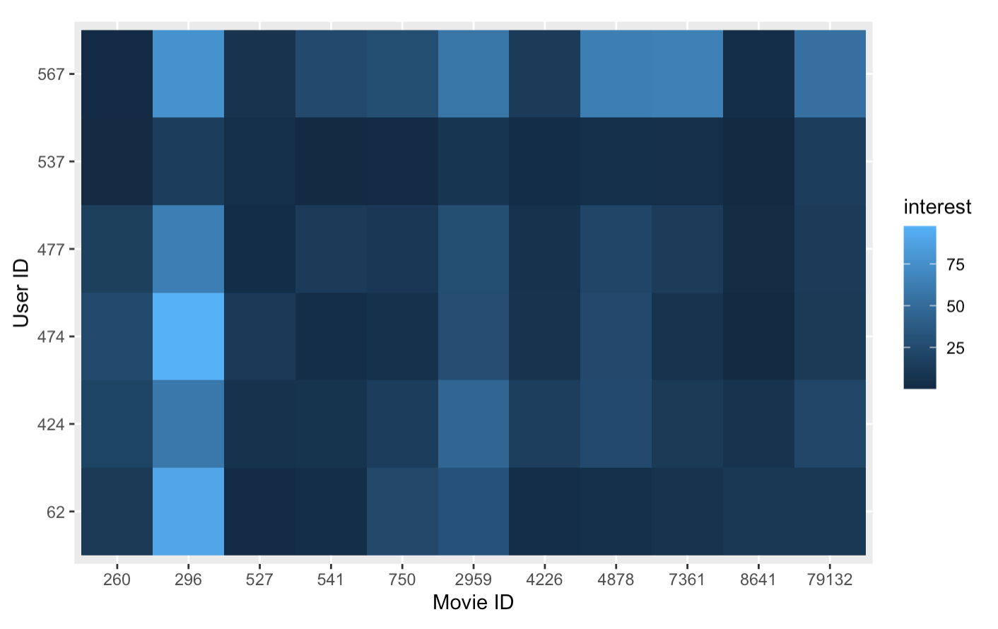
Tag-based recommendation can help us predict the user’s interest on a certain movie. The algorithm’s validity relies on amount of tags. Therefore, when trained on datasets with ample data of tags, the algorithm will become more accurate.
The algorithm penalizes popular tags and popular movies to generate more personalized recommendation results.
Discussion
Explorotory Data Analysis
Key finding & insights
Our exploratory analyses generated an overview of dataset, and helped us to answer most of our initial questions.
We found movies which received most 5-star ratings, and discovered the top 5 popular and highly-rated movies. The Shawshank Redemption (1994) was the most popular film, with 153 times of 5-star ratings. No. 2 Pulp Fiction (1994) had received 123 5-star ratings. Forrest Gump (1994) came in third position with 116 5-star ratings. The Matrix (1999) was ranked fourth among the top five most popular films, with 109 times of 5-star rating. Star Wars: Episode IV - A New Hope (1977) was ranked No. 5 with 104 5-star. We also discovered an intriguing fact: three of the 5 movies were released in 1994, while four were released in the 1990s.
Besides, we also got rating distributions among genres and movie release years, and noted a trend that From 1990 to 2018, the average rating score of movies has become more and more “similar”. That is, the rating values of modern movies are more frequently concentrated between 3.5 and 4, and the density of corresponding scores is close. However, compared to the modern movies from 2000, the user preference for movies from the 90s is more divided, and the density between different ratings is more obvious.
We also performed Kruskal-Wallis Test, whose result suggests significant differences in users’ ratings.
Additional Analyses
Finding Differentiable Movies
Through adaptive bootstrapping, we found the most “differentiable” movies in the dataset. We noticed that these movies are basically high-rating movies. This may be resulted from the trend that movies received more ratings tends to be high-rating movies. However, for high-rating movies, most people love them and only a small proportion of people dislike them. The unbalanced population sizes of lovers and haters may affect the calculation of variance of ratings, as a larger population generally has lower variance compared to smaller population, which can subsequently affect the power of \(D(m)\) in measuring differentiability. So, such result suggests potential bias caused by our method of filtering popular movies. To avoid such problem, if given a dataset with ample records of ratings, we can further filter popular movies to only include those with balanced population of lovers and haters.
Considering timepoint of rating
In our analysis, we excluded the variable timestamp, which describes the timepoint that the rating was given at. However, integration of timepoint may significantly improve the performance of models, because a user’s taste may change with time and does not always stay the same. To integrate timepoint, ratings can be adjusted by timepoint, making ratings given earlier become smaller to reward recent ratings as they reflect users’ current taste.
Tag-based recommendation
A tag-based recommendation system can calculate a numerical value by algorithmically visualizing a user’s interest in a movie. Based on the user’s tag set and the tag set of a specific movie, the system calculates the interest value of the movie and recommends the movie to the user based on this value. The molecule of the formula, which is \(\sum_{b} n_{u, b} n_{b, i}\), firstly compute the user’s interest in a certain movie by finding the sets. \(B(u)\) is the set of tags that user u has labeled, \(B(i)\) is the set of tags that movie i is labeled, \(n_{u, b}\) is the number of times that the user u has labeled tag b and \(n_{b, i}\) is the number of times that movie i has been labeled tag b
However, this formula tends to give a lot of weight to popular movies corresponding to popular tags, which will lead to recommending popular movies to users, thus reducing the novelty of the recommendation results. To solve these problems, scholars improve this formula by drawing on the idea of TF-IDF and constructing the new formula.
\(p(u, i)=\sum_{b} \frac{n_{u, b}}{\log \left(1+n_{b}^{(u)}\right)} \frac{n_{b, i}}{\log \left(1+n_{i}^{(u)}\right)}\),
where \(n_b^{(u)}\) records how many different users have used tag b, \(n_i^{(u)}\)records how many different users have tagged the movie i. The denominator of the formula is used to appropriately punish popular labels and popular items, but the results will not reduce the offline accuracy of the recommendation results while enhancing the personalization of the recommendation results.
Although we got the interest function of user u on movie i, it was still hard to create the heat map. The main problem was the small dataset. The dataset only contains 58 users and most of them only labeled 1 movie. In this way, if the sample size is not large enough, \(n_{b, i}\), which is the number of times that movie i has been labeled tag b, will always be 0. Then we cannot predict the user’s interest anymore and the heat map then will be bad and doesn’t contain useful information.
Luckily, there are several movies that are popular and some users are active. That is, the movies were labeled by several users and some users labeled numbers of movies. We selected the popular movies and active users and then created a heat map.
It is confirmed that if the sample dataset is large enough, then a person will be able to get the interest of any user for any movie and form a movie recommendation system based on it. For example, the interest value is held, and the movie is recommended to the user if it is larger than a certain standard value; the users with similar movie watching interests can be grouped together, and the movie with the highest interest value in this group of users’ will be recommended. In this project, because of the limited sample dataset, time and experience, we could not go deeper. A further investigation can be done in the future.
Shiny app
We implemented results of adaptive boostrapping and user-similarity based recommendation in our shiny app. Users can rate on adaptively-provided movies found by adaptive boostrapping, or rate on any other movie released after 1990. After rating on at least 3 movies, user can get movies recommended by the user-similarity-based recommendation algorithm. The computation for generating recommendation usually takes 1~3 minutes.